OT Salary Analysis
One of my friends is studying occupational therapy (OT), and took a survey with lots of data pertaining to OT salaries. This was data submitted to OTsalary.com where users could download the data and perform their own analyses. The site shows basic analyses such as finding the mean from a spreadsheet, but I decided to take a deeper exploratory approach to the data. The original dataset consisted of 2376 raw survey responses.
The hover functionality is available in the jupyter notebook linked in this github responsitory.
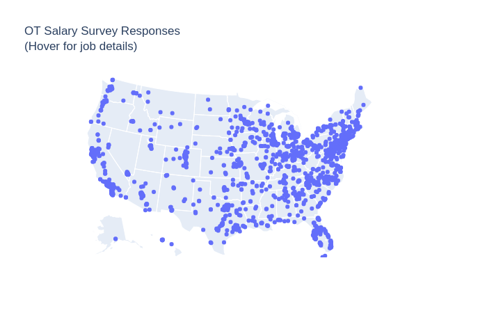
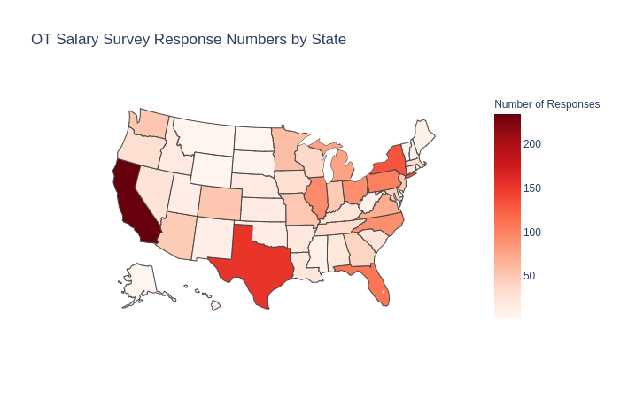
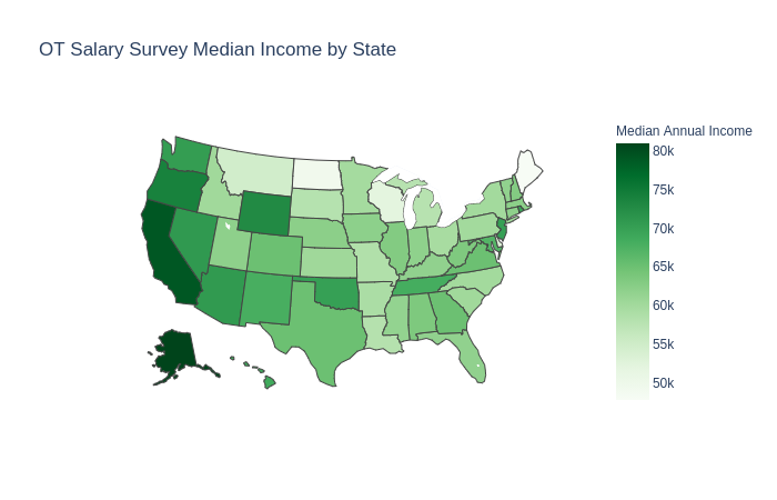
Exploratory Data Analysis
Preliminary EDA showed inconsistencies in the input. For example, there were several instances where annual salaries were much larger when compared to their per hour pay. Conversely, there were salaries extremely low with very high per hour pay. Other issues were inputting numbers such as “74” for salary to possibly indicate 74k or 74,000, or not specifying currency when the responses were international. Overall, these responses were omitted. I also restrict this analysis to US responses, as those were a significant majority of the responses. This results in a dataset of 2176 responses.
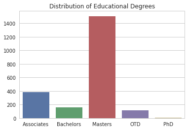
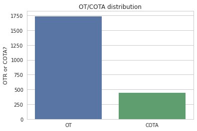
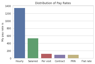
If we split the data into groups, we can see the different class distributions. We look at education, type of OT, location, and type of payrate.
Analysis of a Gender Wage Gap
With these salaries, I wanted to determine whether or not there was a gender wage gap. Spoiler: there is.
We begin by omitting responses that did not prefer to list their gender. We also compare individuals with the same education (masters degrees) and are OTs, because that group consists of the largest number of people. This totals to 114 male responses, 1234 female responses, and 1348 total responses. We can calculate the mean and variance of the salaries, and then apply statistical tests to both.
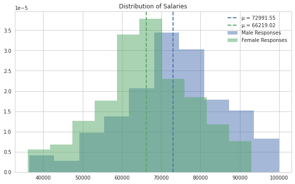

On average, men make $72,991.55 and women make $66,219.02. The difference is $6772.53. This difference of the means is statistically significant, and we can see that by using both statistical tests as well as a permutation test. Our null hypothesis is that the difference of means is 0. Our alternate hypothesis is that they are not equal. (We could assume a one-sided test if we wanted to only see if women make less than men, but we choose the two-sided test for fairness to both genders.)
A Shapiro-Wilk test on the distribution of female salaries shows that it’s not gaussian, but with Levene’s test applied to both distributions, we see it’s homoscedastic (similar variance). With a large enough sample size we apply a two-sided t-test. This results in a p-value on the magnitude of 1e-08.
Permutation Test
We observe the same scenario when applying a permutation test to the data. We use a random sampling version of the permutation test for 20,000 iterations. By randomly shuffling the data, and calculating the means for the randomly shuffled groups, we can generate a histogram of the difference of means that approaches a gaussian distribution. This emulates what the difference of means would be if the two sets of data actually came from the same distribution.
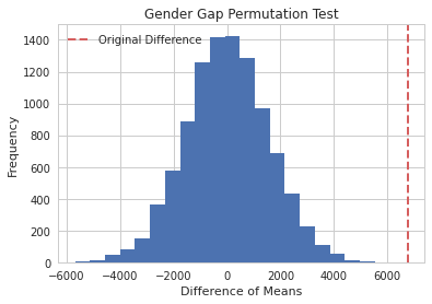
By plotting the observed difference of means on this graph, we can see what are the random odds of observing that original difference. In this case, there were no data points from our permutation test that reached the original difference, thus our conclusion from the permutation test is that we have a p-value of 0. This closely resembles our result from our statistical t-test.
With both tests reaching the same conclusion, we can determine that from this dataset, female OTs with a masters degree make 9.28% less than male OTs with the same level of education.
Salary Prediction
Decision Tree Model
With the data, I used XGBoost to create a gradient boosted decision tree model to predict the salary given a series of inputs. The input data to the tree is a vector with gender, type of OT, state of work, city-type (urban, rural, etc.), and type of pay (salaried, part time, etc.) as one-hot encoded vectors. Years of experience and education are given as ordinal numeric inputs.
The hyperparameters for the XGB regression model is specified in the jupyter notebook. With an 80-20 split on the data, the model has an RMSE of 13,979.83, and an R^2 of 0.464 which shows moderate correlation.
To optimize the hyperparameters, we apply randomized grid search to the gamma, colsample_bytree, subsample, reg_alpha, reg_lambda, learning_rate, and max_depth hyperparameters. We take 500 randomized points and select the optimal model which resulted in an MSE of 13,272.16 and an R^2 of 0.517. This is a slight improvement over the original model.
Visualizing the Tree Model
We can take our decision tree model and graph the splits. As this is an ensemble method, we have many trees working together. One such tree is shown.

The node ‘f60’ corresponds to whether or not the job is part-time. ‘f64’ corresponds to Years of Experience. ‘F56’ is whether or not the person lives in a town. ‘f22’. corresponds to the state ‘MD’ or Maryland. ‘f61’ is if they have a per-visit type of pay, and ‘f42’ corresponds to the state ‘SC’ or South Carolina.
References
Data taken and analyzed from otsalary.com